Principles of Fixed Point Algorithms – Theory and Practice

A fixed-point algorithm is easy to explain: Given a fixed-point function $f$ suited to your problem, choose any point $x_0$ from $dom(f)$ and compute $f(x_0)$ to obtain the next point $x_1$ . Proceed until find point $x_k = f(x_k)$ .

In the following, we expose the conditions in which this strategy works and the reason why. The famous gradient-method can be seen as a fixed-point algorithm.

A simple example

Let’s say you have $n$ pairs of socks that are initially stored in $n$ different drawers. The drawer in which the pair $s$ is stored is given by $d(s)$ . Let’s assume that we start with $d(s)=s \quad \forall s$ . Now we wish to change the drawers of each pair $s$ such that $d(s) \neq s \quad \forall s.$ . Is it possible? Sure it is!

$d(s) = \left\{ \begin{array}{ll} s+1 & s < n\\[0.15in] 1 & s=n \end{array}\right.$

The function $d$ is a permutation and it does not have any fixed-point, i.e., there exists no $s$ such that $d(s) = s$ . Functions with no fixed-points can be generated similarly for any countable set (See Hilbert’s Hotel). Let’s see what we can do with uncountable sets.

If the set is unbounded a similar argument to the one above also holds, so further assume our set is bounded, let’s say $1 < s < 2$ . But once more we can devise a function with no fixed-point with a little bit more of effort. The key point here is that this domain has neither a maximum nor a minimum point. Try to get the largest value in this set, let’say $1.9999$ . You can always get a larger value by adding one more decimal place at the end of the number with a value of $9$ (or $1$ ), for example. Hence, the same shifting idea in the last example applies here. The lowest number with the property of being greater than all others is the number two, but two is not in our domain. Similarly, the highest number with the property of being lesser than all others is the number one, which also doesn’ belong to our domain.

We need to strength our assumptions even more. Let’s impose that every number in our domain in which we can get arbitrarily close must belong to our set. In other words, in the example above, we are asking one and two to belong to our set, namely, we should consider the domain $1 \leq 1 \leq 2$ . A set with this property is called a closed set.

Let’s recall our assumptions: We ask for a uncountable, bounded and closed domain (If you are wondering about closed and unbounded sets, think of \mathbb{R}). Can we now devise a function $d(\cdot)$ with no fixed-point? Yes, we still can!

$d(s) = \left\{ \begin{array}{ll} s+1 & 1 \leq s < n-1\\[0.15in] n-s+1 & n-1 \leq s \leq n \end{array}\right.$

The missing assumption is continuity. We want that every point $y$ close to a point $s$ is mapped to a value close to $d(s).$ Formally:

For every $\epsilon > 0$ there exists $\delta > 0$ such that, for every $z \in (s-\delta,s+\delta)$ implies $|d(s)-d(y)| \leq \epsilon.$

Fundamental results

Brouwer’s Fixed-Point Theorem (for the real line): Let $f:E \rightarrow E$ be a continuous function in which $E \subset \mathbb{R}$ is bounded and closed. Then there exists a point $x \in E$ such that $f(x) = x$ .

The theorem can be generalized for functions of a subset $E \subset \mathbb{R}^n$ , but we need to impose convexity on $E$ . In order to see why note that there is no fixed-point in a 45-degrees rotation of a circle, but we indeed have a fixed-point on a 45-degrees rotation of a ball. Putting differently, the domain $E \subset \mathbb{R}^n$ must be homeomorphic to the unit ball in $\mathbb{R}^n$ .

Brouwer’s Fixed-Point along with Hairy Ball, Borsuk-Ulam and Jordan Curve, are the key theorems to characterize the Euclidean Space.

There exist many fixed-point theorems. To name a few:

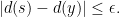
Brouwer’s fixed-point theorem, however, doesn’t give us any hint on the uniqueness of the fixed-point and how to find it. In this sense, Banach’s fixed-point theorem can help us. First, we need to define what is a contraction map:

Definition: A map $f:A\rightarrow A$ is a contraction map on $A$ if there exists a constant $0 \leq q < 1$ such that:

$|f(x)-f(y)| \leq q \cdot (x-y) \quad \forall x,y \in A$ .

In other words, the map $f$ is a contraction map if it is Lipschitz continuous with Lipschitz constant $0 \leq q < 1$ . Lipschitz continuity is a stronger form of uniformity continuity.

Lipschitz Continuous (LC) $\subset$ Uniformly Continuous (UC).

Recall that continuity asks a $\delta$ for every $\epsilon$ and for every $s$ in the domain. In other words, a function $\delta(\epsilon,s)$ must be provided in the general case. For uniformly continuous functions, a $\delta$ that works for a given $\epsilon$ also works for every $s$ in the domain, i.e., we simply need to define a map $\delta(\epsilon)$ . Lipschitz continuous functions are precisely those uniformly continuous functions in which this map is linear. We can also say that a Lipschitz function $f$ with constant $q$ implies $|f^\prime (x)| \leq q \quad \forall x \in dom(f)$ , i.e., its first derivative is bounded.

Examples of Lipschitz Continuous functions:

$\sin,\cos$ in all $\mathbb{R}$ .
$f(x) = ax + b$ in all $\mathbb{R}$ .
$\sqrt{x^2+a}, \quad a>0$ in all $\mathbb{R}$ .
$x^p, \quad p \geq 1$ in $(-3,5)$ .

Examples of Uniformly Continuous functions that are not Lipschitz:

$\sqrt{|x|}$ in all $\mathbb{R}$ .
$|x|\sin{(1/|x|)}$ in all $\mathbb{R}$ .

Banach’s Fixed-Point Theorem (for $\mathbb{R}^n$ ): Let $f:E \rightarrow E$ be a contraction map in $E$ in which $E$ is a bounded and closed subset of $\mathbb{R}^n$ in $\mathbb{R}^n$ . Then there exists a unique point $x^\star \in E$ such that $f(x^\star) = x^\star$ . Moreover,

$\displaystyle x^\star = \lim_{n\rightarrow \infty}{ \big\{ f(x_n) \big\} }$ , with $x_0 \in E$ arbitrary.

Banach’s fixed-point theorem can be generalized for complete metric spaces, i.e., spaces in which every Cauchy Sequence converges to a point that belongs to the space.

One use of the fixed-point theorem is to create a function in which its fixed-point is the solution of a problem one wants to solve. As an example, suppose one wants to compute the root of a function $f(x) = 0$ . It is easy to devise a function $g(x)$ in which its fixed-point is the solution of the problem:

$g(x) = x - f(x).$

The difficulty is that it is not always the case that the devised function holds all the necessary properties of Banach’s theorem, so in practice, convergence proofs of the method should be given by other means.

The oldest application

The oldest applications (although with a rather informally idea behind) of the fixed-point concept is the Babylonian method for computing the square roots.

Let’s say that we want to compute the square root of $a = (x^{\star})^2$ . We start with a wild guess $x_0$ . If $x_0$ is an overestimator of $x^\star$ , then $\frac{a}{x_0}$ is an underestimator of $x^\star$ :

$\begin{array}{ll} \displaystyle \frac{a}{x_0} &=\displaystyle \frac{(x^{\star})^2}{x_0}\\[0.2in] &\displaystyle \leq \frac{(x^{\star})^2}{x^\star}\\[0.2in] &\displaystyle= x^\star \end{array}$

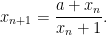
One can devise a better guess by taking the average of the overestimator and the underestimator. The repetition of this procedure gives raise to the Babylonian method.

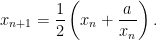
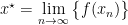
$\displaystyle x_{n+1} = \frac{1}{2}\left ( x_n + \frac{a}{x_n} \right ).$

One can show that the sequence produced by the Babylonian method indeed converges to $\sqrt{a}$ , but it will be useless trying to do so using Banach’s theorem, as Banach’s guarantees us that the Babylonian iterative function will converge only if it is defined in the set $[\sqrt{a/3},a]$ . The fixed-point iteration given by the Babylonian method is by no means the only one available. Many others can be derived, as for instance:

$\displaystyle x_{n+1} = \frac{a+x_n}{x_n + 1}.$

Some of them work better than others, and it is an art to find the best of them. We are going to derive an iterative function guaranteed to converge by Banach’s theorem to the the square root of any number $a \geq 1$ .

$\begin{array}{ll} & x^2 = a \\[0.15in] \Leftrightarrow & (x+k)(x-k) = a - k^2 \\[0.15in] \Leftrightarrow & \displaystyle x = \frac{(a-k^2)}{(x+k)} + k. \end{array}$

We have that $\displaystyle f^\prime (x) = \frac{k^2-a}{(x+k)^2}$ . Hence,

$\begin{array}{ll} f^\prime (x) < -1 & \Rightarrow (a - k^2) > (x+k)^2\\[0.15in] f^\prime (x) > 1 & \Rightarrow (k^2-a) > (x+k)^2. \end{array}$

Then it follows that, if we set $k = a$ and define the function $f(x)$ on the domain $[0,a]$ , the function $f(x)$ is a contraction map and Banach’s theorem tells us the method will converge to $\sqrt{a}$ .

Principles of Fixed Point Algorithms – Theory and Practice

A simple example

Fundamental results

The oldest application

Further reading

Leave a comment Cancel reply

Published by Daniel Martins Antunes

A simple example

Fundamental results

The oldest application

Further reading

Partager :

Leave a comment Cancel reply

Published by Daniel Martins Antunes